The Tech Behind Eon: Scene Packing
This post describes the 3D scene packing and playing in our A500 demo Eon.

Background
Early on we had the idea to precalculate impressive 3D data and render it at a scale that hadn’t really been done on the A500 before. Some demos use versions of the technique described here to draw limited graphics, but we wanted to drop some serious wow moments using this technique and needed something that would allow us to pack a lot of 3D into a small amount of memory.
How we wanted to render stuff
The A500 is not fast enough to do anything like this with polygons transformed in realtime. Instead, what we wanted to do is just store precomputed, closed outlines that we could rasterize and then fill using the blitter. We needed three bitplanes so that we could have the artists flat shade in interesting ways and apply limited lighting effects in some scenes.
Computing contours?
So then the question became, how would we compute these closed contours we needed to draw, and could we squeeze that data down enough to make it work with the very limited space we could allow on the floppies?
False starts and failures
I wrote many versions of this tool over the years the project ran, and it wasn’t until after a couple of years we landed on a version that actually had a shot at working like we needed.
To quickly summarize the things that didn’t work, here they are:
- Image based line reconstruction
- Image based line reconstruction, with brute force search space reduction
- Traditional geometry pipeline with double coordinates
- Off the shelf 2D polygon clipping libraries (we tried many)
We finally gave up on off the shelf clippers and wrote our own version as everything we tried had stability issues with the kind of data that appears in most of our complex scenes.
A breakthrough in the development of our own clipper was the realization that every output vertex (clipped, intersected or normal) will lie at the intersection of two canonical edges, i.e. edges from the input triangles. We store all vertices this way when we build the leaf storing BSP so that ambiguities can be resolved correctly in many more cases than is possible with just numeric coordinates. This made the output geometry much more stable and less prone to leaking and cracking.
Our production version
The production tool uses the following algorithm to process a scene:
- The polygon data is fed through a traditional 3D BSP to generate non-overlapping geometry
- We traverse the data in 3D BSP front-to back order and build a solid leaf-storing 2D BSP tree. Any geometry that falls inside a solid leaf is discarded.
- We apply various voodoo to glue vertices together
- We walk the edges in this BSP tree to build a set of connected contours
- The colors are reshuffled based on bitplanes used so that CPU line drawing will be cheaper
- The data is delta packed
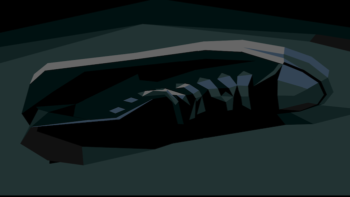
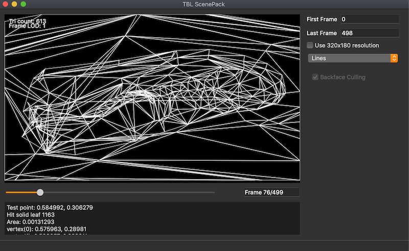
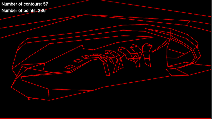
Here is a gallery showing a test scene with various debug modes active:
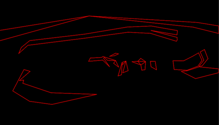
Geometry authored in Maya or Blender:
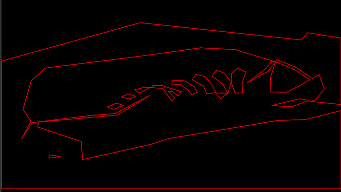
Input triangle soup after 3D BSP splitting:
Output contours (all three bitplanes):
Bitplane 0 only:
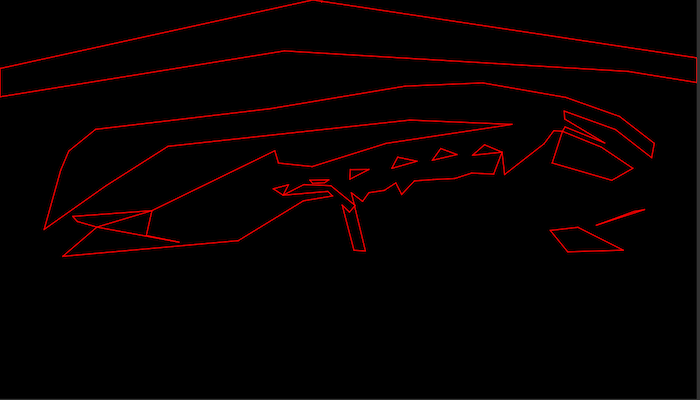
Bitplane 1 only:
Bitplane 2 only:
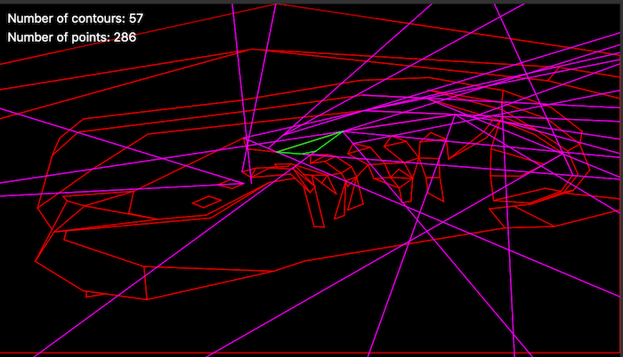
Debugging the 2D leaf storing BSP by selection:
There is also a full profiler built in which kicks the emulator in cycle-accurate mode so artists can work with a scene and optimize it to get it into frame without programmer involvement.
Data stream compression
The basic idea to reduce the size is to try to express the next vertex in a contour as two 6-bit quantities that represent an offset from the previous point. This saves 4 bits per vertex compared to a screen offset.
The output stream is organized by data type. In general this is a good idea to try with any data compression problem, and it certainly helped here to. We output six parallel bit streams which are segmented per frame. Each frame contains the number of bits to consume to render the next frame.
Briefly, the streams are:
- Control stream - contains individual bits indicating yes/no decisions in the decoder
- Count stream - contains runs of counts of vertices (both fully specified and delta encoded)
- Delta stream - contains 6-bit signed offset values for delta encoded vertices
- Full position stream - contains 16-bit numbers which are interpreted as linear screen addresses (this saves one bit compared to basic x/y pairs as x is 0-319)
- Bitplane mask stream - what bitplanes each contour should render to
- Color permutation stream - data to mutate runtime palette order to match encoder decisions
This segmentation per type boosts the additional compression gains we get from LZ4 on top of the data.
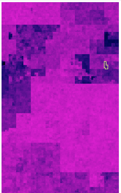
A good way to judge how well data is compressed is to look at a measurement of entropy. This is part of our second floppy as visualized by binvis.io. Purple means close to random and black is predictable:
Playing it back
The blitter is fast enough to clear 3 bitplanes at 320x180 and fill three bitplanes at 320x180 at 25 Hz, but that doesn’t leave enough time to draw the actual lines with the blitter. So we do that using the CPU. We will do a separate post the details the line rendering.
The high-level logic in the render loop looks something like this:
Clear bitplanes
Decode all vertices for the next frame
Mutate palette according to encoded order
Decode 3-bit bitplane masks for each edge
For each contour:
    For each bitplane in masks:
        Draw line from decoded vertex buffer
Fill all bitplanes using blitter
We use quad buffering to make sure that clearing, filling, line drawing and displaying can happen in parallel.
Decoding vertices
Our most common case is runs of 6-bit delta-encoded vertices. So we have longish spans of 6-bit data that needs to be sign extended and converted to 16-bit data. If we look at three bytes, we can see that four 6-bit quanties can fit in the 24 bits exactly:
AAAAAABB BBBBCCCC CCDDDDDDD
This leads to a neat little inner loop possibility that uses a series of lookup tables to transform each byte to the correct value:
.aligned_loop:
	    moveq.l	#0,d2
	    move.b	(a0)+,d2	; aaaaaabb
	    add.w	d2,d2
	    add.w	d2,d2
	    move.l	(a3,d2.w),d2
	    move.w	d2,(a2)+	; write A corrected
	    swap	d2		; swap d2; use high bits as correction for next step

	    moveq.l	#0,d3
	    move.b	(a0)+,d3	; bbbbcccc
	    add.w	d3,d3
	    add.w	d3,d3
	    move.l	(a4,d3.w),d3
	    add.w	d3,d2		; correct partial result from previous iteration
	    move.w	d2,(a2)+	; write B corrected
	    swap	d3

	    moveq.l	#0,d2
	    move.b	(a0)+,d2	; ccdddddd
	    add.w	d2,d2
	    add.w	d2,d2
	    move.l	(a5,d2.w),d2
	    add.w	d3,d2		; correct from previous iteration
	    move.w	d2,(a2)+	; write C corrected
	    swap	d2
	    move.w	d2,(a2)+	; write D corrected

	    dbra	d6,.aligned_loop